For the most part, we have been considering waves in 1 dimension – along a string, down a tube, along a metal bar. Of course, in reality, everything moves in 3 dimensions. However, it is a bit easier to first consider what changes as we go from 1 to 2 dimensions. Also, as mentioned before, there are some musical instruments based on 2-D vibrations, including the cymbals and all drums.

In this section, we will focus on sound waves in 2-dimensions.

When we discussed sound waves in 1-D, we considered a tube. In this case, the diameter of the tube was much smaller than the length of the tube, so it was pretty clear that the sound waves would travel up and down the length of the tube:

To define a 2-D wave, we need a thin rectangular shape:

This is called an acoustic cavity. A cavity is anything that confines waves to a well-defined geometry. Here, the waves again travel in the long directions, and are, thus, restricted to a 2-D plane. From now on, it will be easier to look at the cavity from the top:

When we discussed the air column, we always took L to be the length of the tube. Here, we need to specify two dimensions, the length, L, and the width, W. To start, we can have the same modes in each direction as we had for a tube. In this case, we will assume that the cavity is closed all of the way around corresponding to closed-closed boundary conditions.

Along the length of the cavity, the modes look just like the first diagram in Section 3.6. The wavelengths will be 2L, L, 2L/3, L/2, … Using f× l = v, the frequencies of these modes are: v/(2L), v/L, 3v/(2L), … nv/(2L), … where n is some integer. A simple way of writing this is the frequency of the n^th harmonic is f_n = nv/(2L).

Along the width, we have modes where the wavelengths are 2W, W, 2W/3, … and frequencies are g_m = mv/(2W). We use m here, because we can have different modes in each direction.

So far, the 2-D cavity looks just the same as two 1-D cavities put together. However, the new feature is that the cavity can have both modes going at the same time. Then the question is, what is the frequency of the overall mode? For example, if we are in the 3^rd mode along the length, its frequency is f₃ = 3v/(2L). If we are in the 5^th mode along the width, then g₅ = 5v/(2W). What is the frequency of the mode consisting of both of these modes simultaneously? This is called a combination mode and it needs two numbers to specify it, n and m. The frequency of the combined mode is designated F_n,m and is obtained by adding the frequencies of the two separate modes according to the Pythagorean theorem:

.

Now that we can find the frequencies of the modes, we need to know what they look like. Let’s start with a simple mode along one direction – the second mode in the long dimension. The mode looks just like a mode along a tube, but spread out in the other direction:

We see antinodes at the edges, since it is a closed boundary condition. Red and blue are the extremes, so those colors represent antinodes. Green shows where the nodes are. Since we have the second mode, there should be two nodes. The upper surface shows the amplitude of the wave, while the lower surface is a 2-dimensional representation of the wave.

Here is what a simple mode in the other directions looks like – the first mode along the short dimension:

Again, we see antinodes at the edges and one node. So far, this is not too different from an air column – the mode is just stretched out in the other dimension. So, the question is: what happens if we have both modes at once? Mathematically, the two modes get multiplied together, but you will understand better by just looking at the mode:

The pattern is now somewhat more complicated, but certain elements are apparent. In 1-D, the most important feature in determining the shape of the modes was the location of the nodes. The same is true in 2-D with a difference. In the three images above, green represents the nodes. However, the nodes are no longer points, as they were in 1-D, the nodes are now lines and are referred to as nodal lines. This is not so surprising – going from 1 to 2 dimensions involves adding a dimension. So, if you add a dimension to a point, you get a line. The nodal lines are useful in seeing the mode, because we simply keep the nodal lines from each mode. Here is a simpler representation of all three modes above, showing just the nodal lines:

Second mode in long direction:

First mode in short direction:

Combination mode:

Notice that in these drawings, the rectangle is a dotted line. This is because the edges of the cavity are NOT nodal lines. The thick solid lines represent the nodal lines. To completely show the mode, we can also draw the individual modes to the side of the rectangle as shown:

Finally, if we know the dimensions of the cavity, we can determine the frequency of the mode. This is a complete description of the combination mode. You will become very familiar with these mode patterns between the homework and the labs.

As usual, one problem with sound waves is that we cannot see them, so things like nodes and antinodes are a little abstract. There is a way to see nodal lines in 2-D waves using what are called "Chladni plates". A Chladni plate is a thin plate of metal cut into any shape, but usually a rectangle or a circle. The plate is vibrated with a mechanical oscillator at a resonant frequency. Finally, fine sand is sprinkled on the plate. Since the plate is vibrating the sand dances around and eventually falls off of the plate. However, if the sand is sitting right on a nodal line, the sand does not move, since there is no motion on the nodal line. So, the sand that stays on the plate collects on the nodal lines, showing them quite clearly. Here are some images of Chladni plates taken from http://www.physics.uiowa.edu/~dstille/acoust/3D40.30.htm:

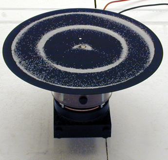
Now, don’t worry, you will not have to be able to draw these nodal lines! The nodal lines on the Chladni plates are quite a bit more complex than for sound waves in a rectangle. This is just like the fact that the modes of vibrating bars are more complex than for air columns. Vibrating metal plates are even harder to describe than vibrating metal bars. However, the Chladni plates are still interesting because they vividly show the reality of the nodal lines.