Gohn -- Log

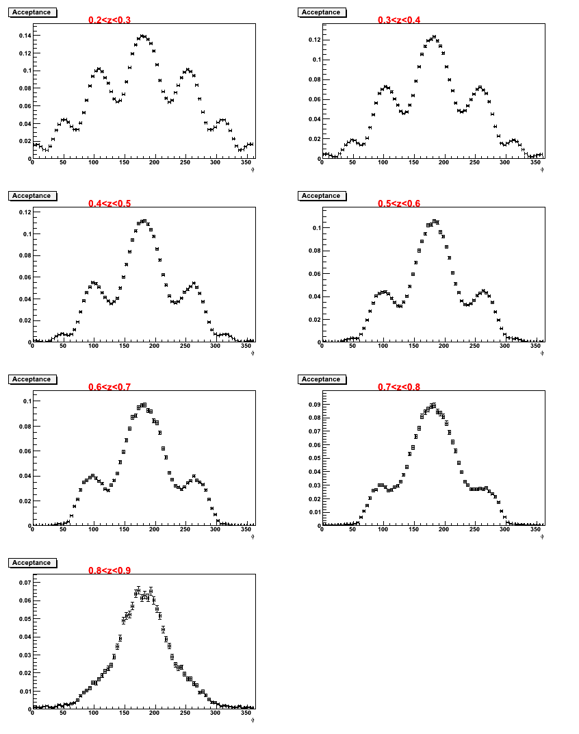
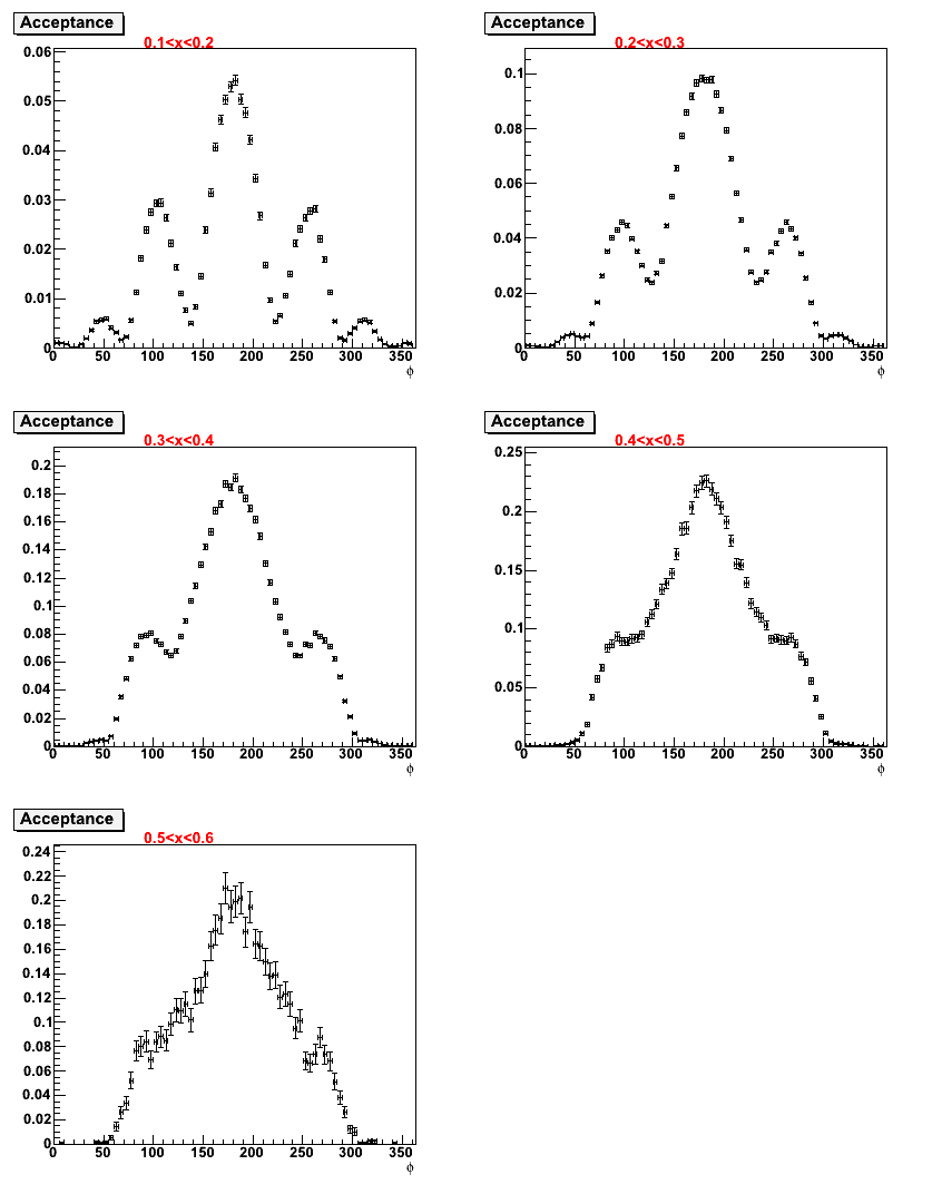
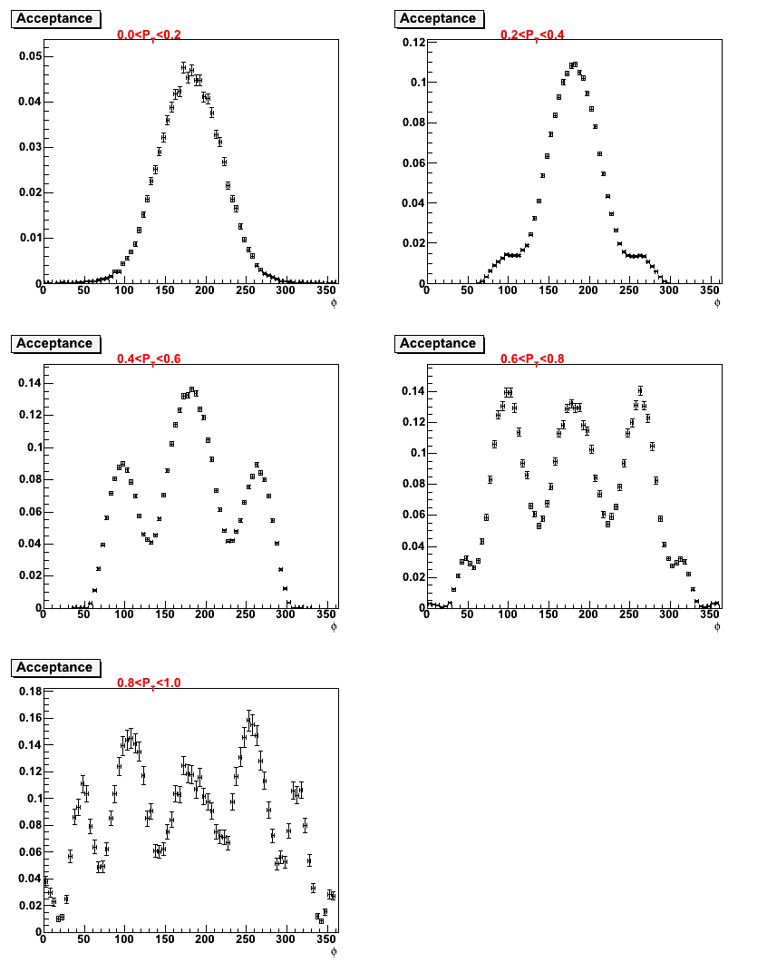
December 6, 2011

I am still working on reproducing the Cahn effect implementation in the event generator in my weighting program. In the event generator, the effect is applied by:

2 continue
phi=rlu(0)*twopi
dstr=y11-cahn1*cos(phi)+cahn2*cos(2.*phi)
if(dstr/cahnmax .lt. rlu(0)) goto 2
phiq=phi
return

Here rlu(0) returns a random number between 0 and 1, which is converted to a random φ by multiplying by 2π. y11, cahn1, and cahn2 are calculated as functions of y, P_T and Q², and cahnmax = y11+cahn1+2*cahn2.

To reproduce the above loop, I impliment it as follows into my own program:

while(dstr/cahnmax < rlu){
rlu = (double) rand()/RAND_MAX;
randphi = rlu*2*PI;
dstr = y11 - cahn1*cos(randphi)+cahn2*cos(2*randphi);
}

Here all quantities are calculated exactly as above. rand() returns a random number between 0 and RAND_MAX, so dividing by RAND_MAX makes it the same as rlu(0) in the Lund function. When the weighting is applied using this function, the weights come out to be completely flat in φ, as can be seen below.

I am currently investigating the following:

rlu(0) is called twice in the Fortran loop. Does it give a different random number each time, or is it somehow fixed for an iteration of the loop?
What is phiq? It seems to not be used again in the program after it is set in the loop. Maybe it is passed into a variable with a different name?
In order for the weight to get a φ dependence, it seems that I should use the random φ as the φ for the event (and maybe this is the phiq?), but this seems like it must be wrong. How can I measure φ dependence if I am not looking at the same φ?

Here the red points are the data applying the weighting procedure above.

December 3, 2011

I am still working on understanding how the Cahn effect is included in the clasDIS event generator. I am using two methods. The first is to go through the clasDIS code to try to better understand how the Cahn effect is included. The second is to go back to the original Cahn paper to see what the analytic function should be.

I have identified a possibility for what I was doing wrong with the weighting method, and I am currently working to properly incorporate that into my weighting procedure. In the clasDIS code, it does not actually weight as a function of φ for the event, but uses a randomly generated φ, and tests to see that the computed weight passes a certain threshhold. I hope that my using the identical procedure in my weighting program, it will accurately reproduce the φ distributions given from the MC. This is still being tested, but I will show results soon.

I hoped that by determining the analytic function of the Cahn effect, this may help to see how the z-dependence is introduced in clasDIS. I have studied Cahn's original paper, and so far the function given by clasDIS does not seem to be in agreement. The following table compares the functions used in clasDIS to that given in the Cahn paper.

	clasDIS	Cahn paper
<cosφ>	4(1-y)^1/2(2-y)P_T/Q	2(1-y)^1/2(2-y)P_T/Q × (1+(1-y)²)^-1z²/(1+z²)
<cos2φ>	4(1-y)P_T²/Q²	2(1-y)P_T²/Q² × (1+(1-y)²)^-1z⁴/(1+z²)²

As you can see, the analytic functions are not the same. Since I am still unsure of how z-dependence is introduced into the MC function, I also compared the analytic curves to the generated φ distribution in fixed bins as was done before. From the plots below, you can see that the Cahn effect intoduced into the program by the MC is significantly larger than that computed based on the function given in Cahn's paper.

November 16, 2011

Using fixed kinematics, I am attempting to determine the z-dependence of the Cahn effect as it is included in the event generator. I fit the distribution in φ due to the Cahn effect in four z bins holding P_T, y, and Q² constant. By fitting the coefficients on the φ function as a function of z, I can estimate the required z-dependence. Many functions of z were attempted, but a 2nd order polynomial has given the closest results.

The first two plots show the coeffictients on cosφ and cos2φ as functions of z, and fit with a 2nd order polynomial.

The next four plots show the comparison of the φ distributions. The black curve is the analytic curve of the Cahn effect using the z-dependence from the above fits. The grey curve is the fit to the φ distribution that is generated with the Cahn effect included.

November 11, 2011

The following are plots of φ for fixed kinematics using the same values of P_T, Q², and y, and two different values of z. The low statistics make it hard to see variations by eye, so the MC data including the Cahn effect are fit to make a comparison. The solid black curve is the analytic function calculated from P_T, Q², and y (It is NOT a fit). Small differences in the analytic function are because the values used for each kinematic variable are the RMS values after the z cuts, so although the cuts on P_T, Q², and y do not change, the RMS can still have a small fluctuation. I am in the prcess of reproducing the two plots below for two different values of z in order to better see the relationship.

November 9, 2011

Below are two plots of the generated φ using very specific kinematics, overlaid with the analysic function of the Cahn effect that is used to weight the flat events. Two kinematic points are compared, both of which show good agreement between the weighted events and the analytic function. The function is a function of P_T, Q², and y. Specific values of P_T and Q² were chosen for each test, and the RMS value of y after the cut is used to compute the Cahn function.

I am in the process of reproducing the above for further fixed kinematic points, including fixed values of z.

November 3, 2011

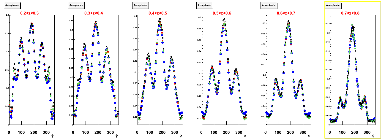
Below is a comparison of φ binned in z for each of the six sectors in CLAS. At first glance there does not seem to be a large difference between the sectors, but when the data is fit it can be seen that the discrepencies between each sector are very large. The plots below use only the flat φ with no weighting, but a comparison using data generated with the Cahn effect and flat data weighted with the Cahn effect is underway.

Uncorrected φ:
Acceptance:
Corrected φ:

October 26, 2011

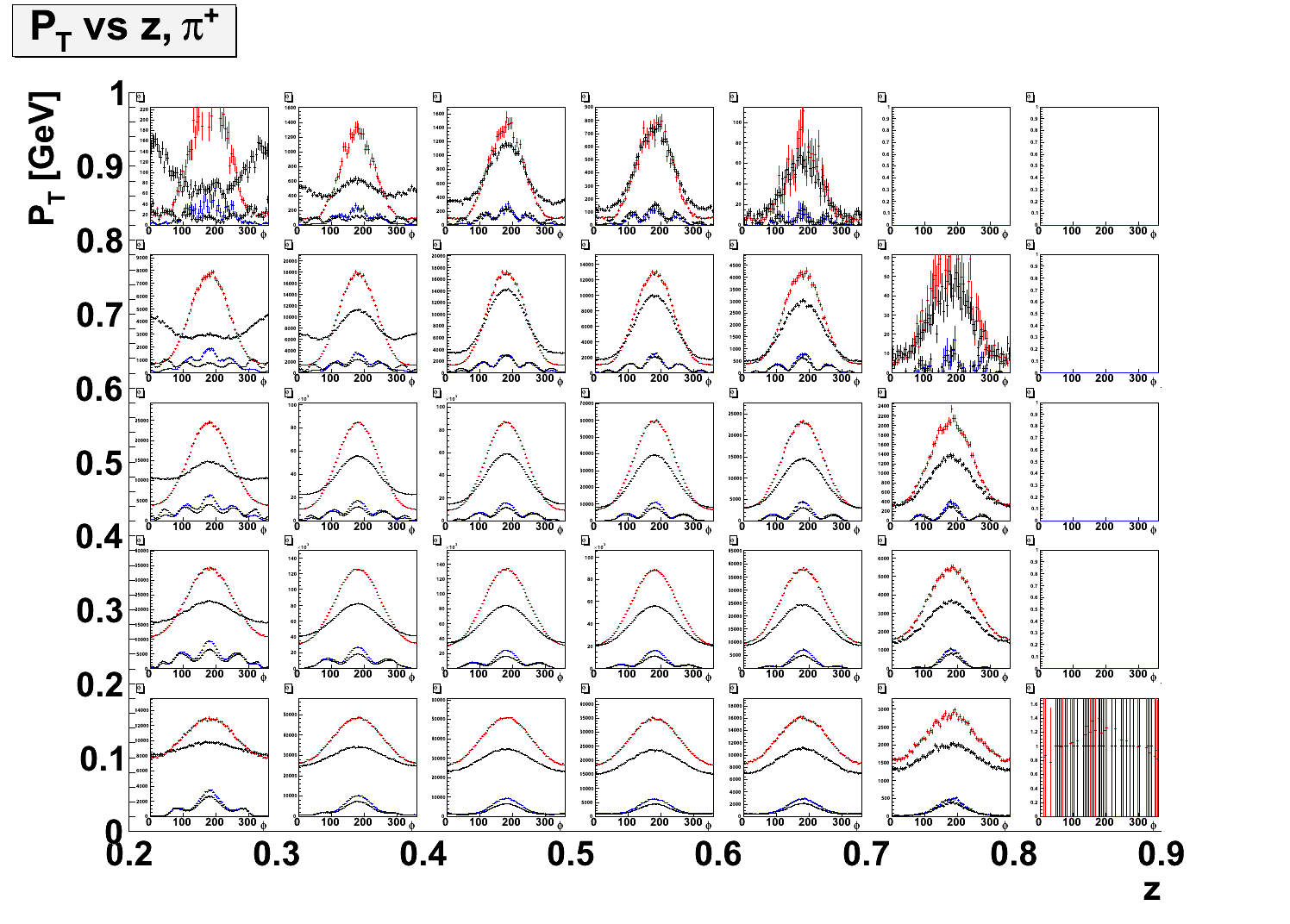
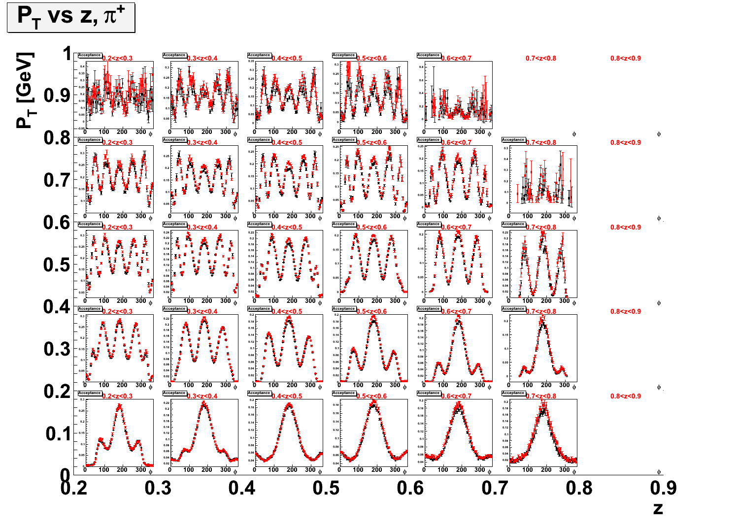
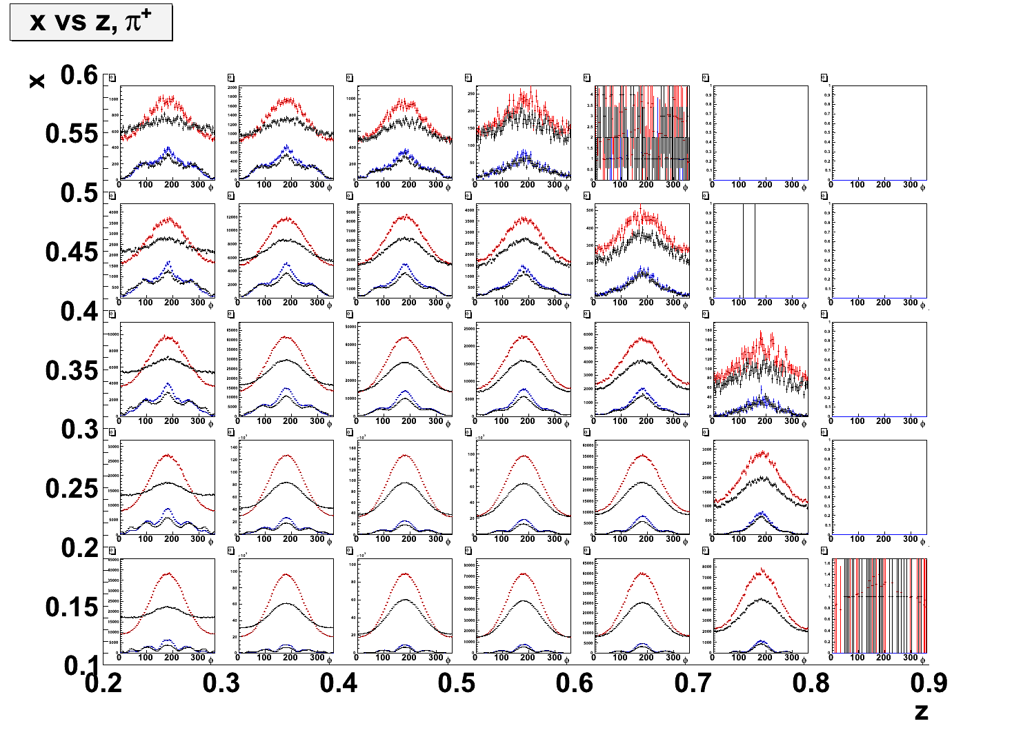
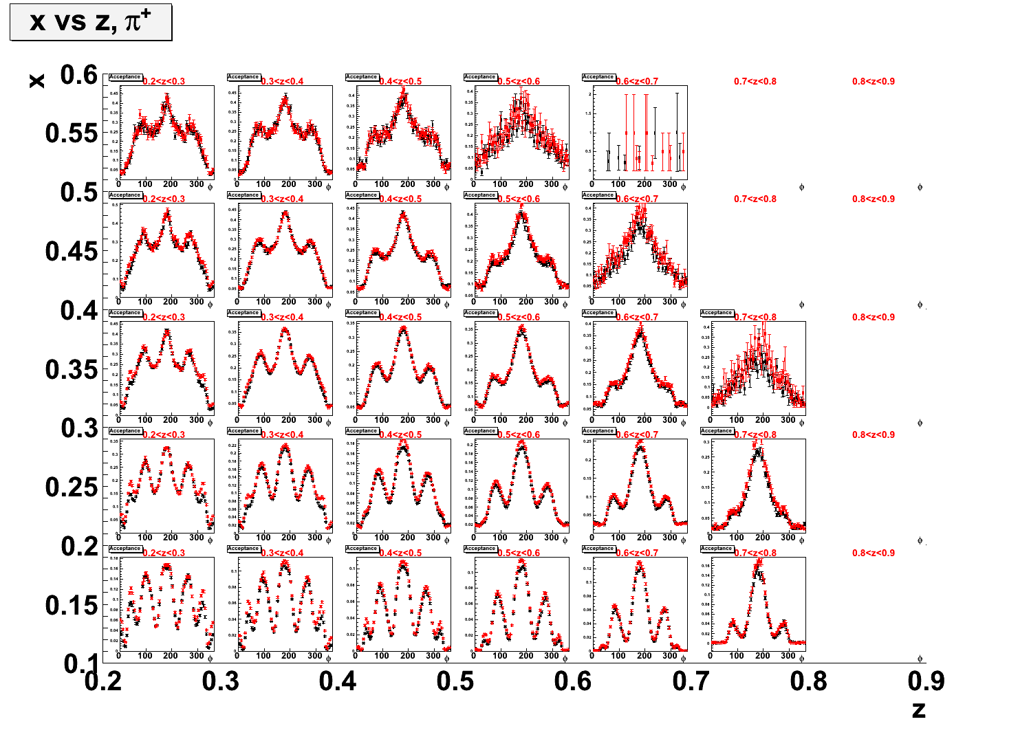
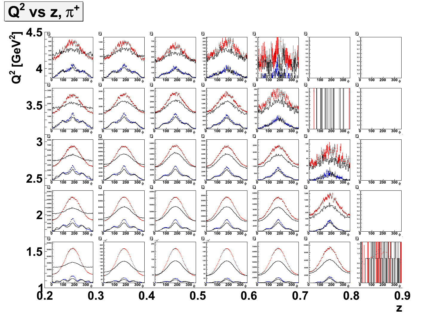
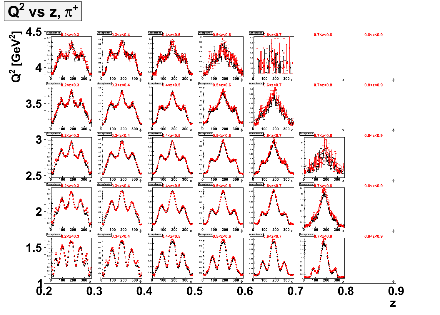
2-dimensional plots comparing simulation generated with Cahn effect and simulation generated with a flat φ and weighted with the Cahn effect. Some bins in x and Q² show some small discrepencies between the two procedures and wide values of φ. There are very large discrepancies between the two procedures are large P_T and low z.
- P_T vs. z. Red/blue = Event Weighting, black = Cahn in generator.
- x vs. z.
- Q² vs. z.
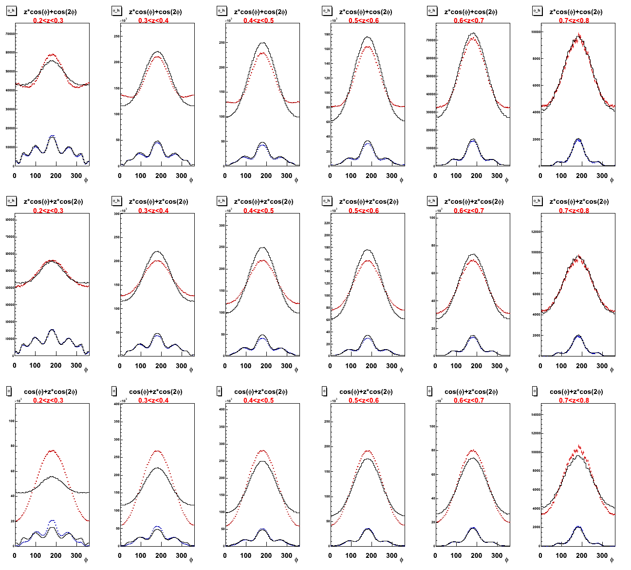
Test of manually adding z-dependence to weighting procedure. Multiplying the cos(φ) term by z provides a large improvement in the matching between the simulation generated with the Cahn effect and that generated with flat φ and weighted with the Cahn effect.

October 25, 2011

I am working on an event weighting procedure to mirror the Cahn routing implemented in the event generator. To do so I weight each event from the flat φ distribution with the following function:
q2pt = pt/sqrt(q2)
q2pt2 = pt**2/q2
y1 = (1.-y)
y11 = 1.+y1**2+4.*y1*q2pt2
y12 = sqrt(y1)
y2 = 2.-y
cahn1 = 4.*y12*y2*q2pt
cahn2 = 4.*y1*q2pt2
weight = y11-cahn1*cos(phi)+cahn2*cos(2.*phi)

Events are weighted with the above function, and then compared to both the flat φ distribution and the MC produced with the Cahn Effect. The events weighted with the Cahn effect compare better with events generated with the Cahn effect than to those with a flat φ distribution, but the systemmatic error between the two fits is still too high. I am working on the weighting procedure to see if it can be improved. In particular, the generated φ distributions are different between events weighted with the Cahn effect and those generated with the Cahn effect, so I am trying to understand this difference.

Comparison to flat φ:
Comparison to Cahn function in the event generator:
- Red is generated with flat φ and weighted with the Cahn effect, and black is generated with the Cahn effect.
- Fits to φ corrected with weighted Cahn.
- Fits to φ corrected with Cahn in event generator.

October 21, 2011

The following are plots showing the weighting procedure for acceptance calculation.

The following shows generated events using each of the three weights. The red (blue) histograms are generated (reconstructed) histograms using the weighting method. The histograms plotted in black are those using a flat φ distribution.
The following are acceptances produced from each of the three weighting procedures and compared to the acceptance calculated from the flat φ (black points):
Here are ratios of each acceptance to that produced from the flat φ distribution.
The remaining are fits to the φ distributions after being corrected by each of the four acceptances (flat and the three weights).
- Flat φ:
- 1+0.05*cosφ:
- >1+0.1*cosφ:
- >1+0.2*cosφ:

October 19, 2011

Today's update contains the following:

Comparison between M_X>1.2 and M_X>1.5 using flat φ
Comparison between flat φ and Cahn effect using M_X>1.5 GeV and y<0.8.
Purity plots using flat φ and Cahn effect.
Kinematic plots using M_X>1.5 GeV and y<0.8.

Using flat φ, comparison between M_X>1.2 and M_X>1.5 GeV.
- Uncorrected φ with M_X>1.5 GeV:
- Acceptance with the two missing mass cuts:
- Ratio of Acceptances with M_X>1.5 and M_X>1.2.:
- Corrected φ using M_X>1.5 GeV and y<0.8.:
Comparison between simulations using flat φ and Cahn effect, both now with momentum-matching, M_X>1.5 GeV, and y<0.8.
- Uncorrected φ:
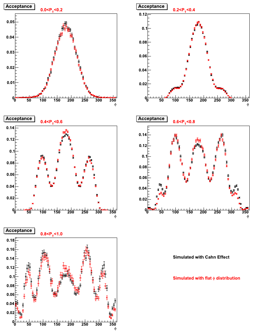
- Acceptance with and without Cahn effect:
- Ratio of Acceptances with and without Cahn effect:
- Corrected φ:
Purity plots using simulation with flat φ and Cahn effect, both with M_X>1.5 GeV and y<0.8.
- Simulation with Cahn effect:
- Simulation with flat φ:
Kinematic plots using cuts on M_X>1.5 GeV and y<0.8.
- Simulated with Cahn Effect:
- Simulated with flat φ:

October 18, 2011

Here are plots of purity, defined as purity in the nth bin = the number of reconstructed events at the same time generated in the nth bin divided by the number of reconstructed events in that bin. The calculation is done in (z,φ) binning using 72, 36, and 18 bins.
Here is acceptance in (z,φ) binnng using the pion momentum-matching.
- Uncorrected φ (unchanged):
- Simulated φ with momentum-matching imposed on reconstructed events:
- Acceptance:
- Ratio of Acceptances with and without momentum-matching:
- Corrected φ:
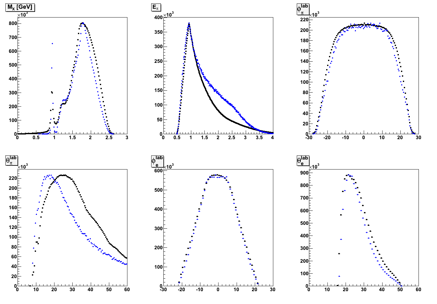
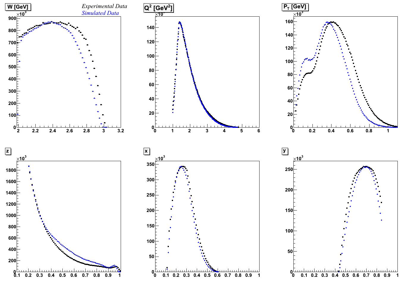
Posted below are kinematic plots after the momentum-matching algorithm is implemented for simulated events. The plots of Q², P_T, and x include the cuts on W>2, Q²>1, 0.4<z<0.7, M_X>1.2 GeV, and y<0.85. The plots of z and E_π include cuts on Q², W and y. Plots of θ and φ use only the particle identification cuts.

October 17, 2011

Below are plots of kinematic variables between experimental and simulated data. There is a large difference in pion θ, as well as small differences in some other variables. I am currently running my analysis program on simulated data using a momentum-matching algorithm to assure that for each event, the reconstructed pion with the highest energy is coming from the generated pion with the highest energy. Tomorrow I will remake the kinematic plots below to see if this matching algorithm provides any improvement. I am also currently creating histograms to calculate the purity in each bin. Next I will perform the weighting analysis procedure.

October 15, 2011

Comparison of acceptance using a flat φ distribution to that using the Cahn Effect in 2-dimensions (z,φ).
- Uncorrected φ:
- Simulated φ with Cahn effect:
- Simulated φ without Cahn effect:
- Acceptance:
- Ratio of Acceptances:
- Corrected φ:
Comparison of acceptance using a flat φ distribution to that using the Cahn Effect in 3-dimensions (z,x,φ).
- Uncorrected φ:
- Simulated φ
- Acceptance:
- Ratio of Acceptances:
- Corrected φ:
Comparison of acceptance using a flat φ distribution to that using the Cahn Effect in 3-dimensions (z,Q²,φ).
- Uncorrected φ:
- Simulated φ
- Acceptance:
- Ratio of Acceptances:
- Corrected φ:
Test of the two acceptance calculations. The acceptance using the Cahn effect is used to correct reconstructed events with a flat φ distribution and vice versa.
- Events simulated with Cahn effect and corrected with acceptance using Cahn effect.
- Events simulated with Cahn effect and corrected with acceptance with flat φ.
- Events simulated with flat φ and corrected with acceptance using flat φ
- Events simulated with flat φ and corrected with acceptance using the Cahn effect.

October 14, 2011

I fixed a bug in my code that was causing the missing mass cut to not be correctly applied. which greatly improved the φ distributions. For the following plots and fits to φ I used the simulation including the Cahn effect. I am currently running the program on the files simulated with the flat φ distribution for comparison.

October 12, 2011

The following show acceptance corrections in three dimensions in terms of (z, x, φ) and (z, Q², φ) using 72 bins in φ.

(z, x, φ)
- Uncorrected φ
- Simulated φ
- Acceptance
- Ratio of acceptances:
- Corrected φ
(z, Q², φ)
- Uncorrected φ
- Simulated φ
- Acceptance
- Ratio of acceptances:
- Corrected φ

October 11, 2011

Plots for π⁺ using 20 degree bins in φ:
- Uncorrected φ from E1-f:
- Simulated φ.
- Acceptance. Red uses Cahn effect and black is flat φ.
- Ratio of Acceptances:
- Comparison of corrected φ:
Plots for π⁺ using 10 degree bins in φ:
- Uncorrected φ from E1-f:
- Simulated φ.
- Acceptance. Red uses Cahn effect and black is flat φ.
- Ratio of Acceptances:
- Comparison of corrected φ:

I also tested the effect of the elctron fiducial cut on acceptance. I used the events simulated with a flat φ distribution, but used a tighter electron fiducial cut. The following plots compare the acceptance due to the two cuts. For this comparison I used 180 bins in φ.

Uncorrected φ distribution from E1-f:
Simulated φ distributions:
Acceptance. Black is original and red uses the tighter cut:
Ratio of acceptance using tight fiducial cut over acceptance using normal fiducial cut:
Corrected data:

October 10, 2011

Here is a comparison of the φ distribution in each z bin after being corrected with each of the two acceptance corrections.

October 6, 2011

These are showing Monte-carlo data that has been reconstructed in GSim, and then corrected with the computed acceptance. We want to see the 2nd row reproducing the 1st row and the 4th row reproducing the 3rd row. I adjusted the range of the fits to only include data points between 30-330^o, ignoring the edges.

The first plot shows data generated with the Cahn effect, and corrected with acceptance including the Cahn effect (returns exactly the generated data).
The second plots shows data generated with the Cahn effect, and corrected with acceptance with no Cahn effect.
Next is data generated with flat φ and corrected with flat φ (returns exactly generated flat φ distribution).
Last is data generated with a flat φ distribution and corrected with acceptance including the Cahn effect.

October 5, 2011

Here is z-dependence for π⁺ using 2^o bins in φ..

Uncorrected φ from E1-f:
Simulated φ with Cahn effect. Red is generated and blue is after GSim.
Simulated φ with flat φ.
Acceptance. Red uses Cahn effect and black is flat φ.
Ratio of Acceptances:
Corrected φ using simulation with Cahn effect:
Corrected φ using simulation with flat φ.

October 4, 2011

Here using 2^o bins in φ (previous plots used 5^o bins).

Uncorrected φ from E1-f:
Simulated φ with Cahn effect. Red is generated and blue is after GSim.
Simulated φ with flat φ.
Acceptance. Red uses Cahn effect and black is flat φ.
Ratio of Acceptances:
Corrected φ using simulation with Cahn effect:
Corrected φ using simulation with flat φ.

October 3, 2011

Uncorrected φ from E1-f:
Simulated φ with Cahn effect. Red is generated and blue is after GSim.
Simulated φ with flat φ.
Acceptance. Red uses Cahn effect and black is flat φ.
Ratio of Acceptances (added on 10/4):
Corrected φ using simulation with Cahn effect:
Corrected φ using simulation with flat φ.

September 29, 2011

Here are fits giving the z dependence of A^cosφ using 40M generated events comparing the two φ distributions.

Flat φ:
With Cahn Effect:

September 27, 2011

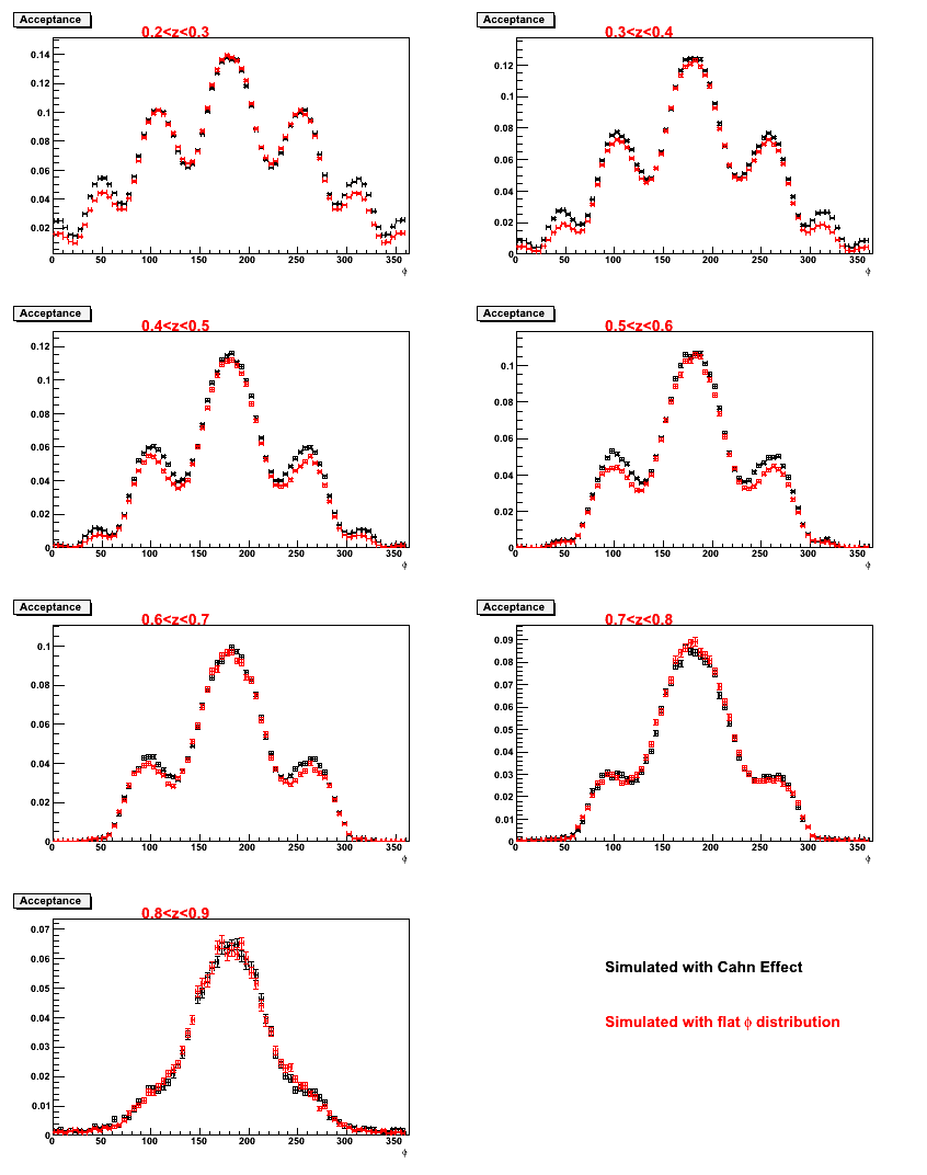
Comparisons of acceptance from the two simulations as function of P_T and z:
Here is a comparison of the kinematics resulting from each simulation. The simulation using the Cahn effect seems to give slightly more events at higher z.

September 26, 2011

I found a bug in my code that was giving incoorect acceptance using the Cahn effect. I fixed it, and replaced the plots posted earlier today. The original plots are here and here. Now the acceptances from the two generated samples are much more similar. Both use 40M generated events.
The first six plots show acceptance in each x bin resulting from data generated using a flat φ and data generated using the Cahn effect.
Here are the generated and reconstructed φ distributions with the Cahn effect included.
Here are fits to the φ distributions using 40M generated events (10% of my total sample) with the Cahn effect included. The minimum acceptance cut is at 2%.

September 22, 2011

Completed Table 4, which divides each value in table 2 by the corresponding acceptance in table 3, and is observed to return exactly table 1 except for bins where acceptance is below 2%, which are set to zero.

September 21, 2011

Have so far created the first three tables that Kyungseon asked for in email earlier today. The the first two show the number of generated and reconstructed events in each bin using the simulation including the Cahn effect. The third shows the acceptance in each bin.
- Table 1: Generated Events
- Table 2: Reconstructed Events
- Table 3: Acceptance
Working on fits to the φ distributions in each x bin corrected with the flat acceptance for π^-. Following Mauri's suggestion I have been testing a minimum acceptance cut. The following fits with different cuts are as follows:
- Acceptance>0.1%
- Acceptance>0.5%
- Acceptance>1.0%
- Acceptance>2.0%

September 19, 2011

Here are plots of acceptance for π^- from the flat φ simulation, each as a function of only one kinematic variable z, x, and P_T with φ_h.

September 16, 2011

A recap of yesterday's meeting is here.
Fit the φ distributions from the event generator with the Cahn effect included, which shows larger values of A^cosφ than I expected. The plots are posted here.
Below is the acceptance calculated in one dimension (φ only) for π^- using the MC with a flat φ distribution.

In the first plot, the red is generated and the blue is reconstructed. The second plot shows the acceptance (or the ratio of the two).

The following plot applies the above acceptance to E1-f π^- data.

September 6, 2011

I am currently creating a set of generated data files for using a flat φ distributions. These are running on the batch farm now.
I have modified my program to match Osipenko's binning in z and P_T to make a detailed comparison using the same bins. The program is running to fill the histograms using this binning.
I have been looking at my acceptance calculation and trying to determine the source of the few bins with very large A^cosφ. I examined each bin in the 4-dimensional binning and compared the reconstructed φ distributions from GSim to those in the E1-f dataset [1], and made a list of bins where the distributions did not match. The bins that do not match all lie in the region of z<0.3 and P_T>0.6. There is no noticable dependence on x or Q². I integrated over x and Q² and fit the data in each z, P_T bin. The results are displayed below, showing a trend opposite to my expectation that the low z, high P_T bins would have very large value of A^cosφ. Instead the magnitude of A^cosφ increases with z.

Also, here is a plot of z vs P_t for GSim reconstructed π^-

August 24, 2011

I have updated my φ fits in 4-dimensional binning and when integrated over Q². The plots are shown here:
- Binned in z, x, P_T and Q²
- Binned in z, x, and P_T
Now working on two sets of 2D binning. For the first I integrate over 0.4<z<0.7 and look at x vs P_T binning, and for the second I integrate over x and bin in P_T and z. The second set I will need for comparison to Osipenko's results.

August 18, 2011

I have posted very preliminary fits for my cosφ and cos2φ moments. The fits shown are using the full 4D binning in x, P_T, z, and Q². I am currently going through bin by bin to improve the fits. I also am testing different binning and seeing how much my fits improve if I integrate over Q² and/or z. The fits are posted here.
I updated the simulated event numbers for π^- here,
Today I gave Peter a revised copy of the theoretical chapter for my thesis.

August 15, 2011

Posted a summary of my simulation so far. I am processing another batch of π^- events to add to this total.
I am working on binning and fitting of the acceptance-corrected φ distributions.
I have been working on an updated version of the theory chapter for my thesis incorporating Peter's comments, which I will send soon.

August 11, 2011

Redid acceptance calculation for π^- with updated code which eliminated the peak at φ=0. The plots on the web have been updated to reflect the change.
I met with Peter again to discuss my thesis chapter and am continuing to edit and add to it. I will send an updated version soon.

August 9, 2011

One the web page showing acceptance plots there is now a button to choose the φ range between 0 to 360 or -180 to 180. I found a bug in my π^- ID code that caused the spike at φ=0. I have corrected this and am running my code to refill the histograms. Plots are located here.

August 6, 2011

Posted five-dimensional acceptance calculation for π^- here. Some bins have a spike in the GSim reconstructed data at φ=0. I am currently working to determine the cause of this spike.
Processed about 35M simulated events on the batch farm.

August 5, 2011

Began working on new calculation of acceptance for π^-
Processed about 35M events on the batch farm.
Peter gave me many suggestions to improve the theory chapter of my thesis, so I am working on implementing his comments.

August 3, 2011

Posted five-dimensional acceptance calculation for π⁺ here.
Batch farm processed about 6M simulated events today.

August 1, 2011

Processed 29M pi- events on the batch farm and prepared another 130M pi+ events to be submitted tomorrow.
Ran analysis program on simulated data, giving 22M reconstructed pi+ events passing the SIDIS cuts (compared to 9M from E1-f data).
Currently working on acceptance calculation for pi+.

July 31, 2011

Over the weekend the batch farm has completed processing 67M π^- events. I have started generating a new batch of π⁺ events to be submitted when this finishes.
Completed pion id for simulated data, as shown below. I am currently running my analysis program over all my simulated data files for π⁺.

July 28, 2011

Finished electron id part of analysis program for simulated data. Working on pion id.
Batch farm processed 2M simulated pi- events today.

July 27, 2011

Finished debugging analysis program for simulated data and am working on updating particle id routines.
Batch farm completed processing of 5M simulated pi- events.

July 26, 2011

Completed 15M simulated pi- events on the batch farm.
Made progress updating new version of analysis program for simulated data.
Finished preliminary draft of the theoretical chapter of my thesis. I plan to go through this with Peter and ask him for any suggestions.

July 25, 2011

My jlab.org website is still not accessible, so I will temporarily post daily updates at this location.
I am almost finished with a draft of my theoretical chapter for my thesis, and will send out the draft soon.
I have been running my event generator to improve the size of my generated data sample. I started a batch of 130M events each of π⁺ and π^-. I have completed about 90% of the π⁺ events, and am currently running the generator for the π^- events, which will be submitted to the batch farm tomorrow.
Since I have made several recent modifications to my analysis program, I am working on testing and updating the newest version of the program to work with my simulated data.